Section 3. An Approach to Selecting Ecosystem Indicators for Puget Sound

Ecosystem indicators are quantitative biological, chemical, physical, social, or economic measurements that serve as proxies of the conditions of attributes of natural and socio-economic systems (Environmental Protection Agency 2008, Kurtz et al. 2001, Landres et al. 1988, Fleishman and Murphy 2009). Ecosystem attributes are characteristics that define the structure, composition and function of the ecosystem that are of scientific and/or management importance, but insufficiently specific and/or logistically challenging to measure directly (Environmental Protection Agency 2008, Kurtz et al. 2001, Landres et al. 1988, Fleishman and Murphy 2009). Thus, indicators provide a practical means to judge changes in ecosystem attributes related to the achievement of management objectives. They can also be used for predicting ecosystem change and assessing risk.

Terminology and Concepts

Indicators	Quantitative biological, chemical, physical, social, or economic measurements that serve as proxies of the conditions of attributes of natural and socioeconomic systems.
Key Attributes	Characteristics that define the structure, composition, and function of a Focal Component.
Focal Components	Major ecological characteristics of an ecosystem.
Goals	Combine societal values and scientific understanding to define a desired ecosystem condition.
DPSIR framework	Driver-Pressure-State-Impact-Response (DPSIR). Drivers are factors that result in pressures that cause changes in the system. Pressures are factors that cause changes in state or condition. State variables describe the condition of the ecosystem. Impacts measure the effect of changes in state variables. Responses are the actions taken in response to predicted impacts.

For more information and links to references, see Glossary.

Ecosystem indicators are often cast in the Driver-Pressure-State-Impact-Response (DPSIR) framework—an approach that has been used by the PSP and broadly applied in environmental assessments of both terrestrial and aquatic ecosystems, including NOAA’s Integrated Ecosystem Assessment (Levin et al. 2008). Drivers are factors that result in pressures that cause changes in the system. Both natural and anthropogenic forcing factors are considered; an example of the former is climate conditions while the latter include human population size in the coastal zone and associated coastal development, the desire for recreational opportunities, etc. In principle, human driving forces can be assessed and controlled. Natural environmental changes cannot be controlled but must be accounted for in management. Pressures are factors that cause changes in state or condition. They can be mapped to specific drivers. Examples include coastal pollution, habitat loss and degradation, and fishing. Coastal development results in increased coastal armoring and the degradation of associated nearshore habitat. State variables describe the condition of the ecosystem (including physical, chemical, and biotic factors). Impacts comprise measures of the effect of change in these state variables such as loss of biodiversity, declines in productivity and yield, etc. Impacts are measured with respect to management objectives and the risks associated with exceeding or returning to below these targets and limits. Responses are the actions (regulatory and otherwise) that are taken in response to predicted impacts. Forcing factors under human control trigger management responses when target values are not met as indicated by risk assessments. Natural drivers may require adaptational response to minimize risk. For example, changes in climate conditions that in turn affect the basic productivity characteristics of a system may require changes in ecosystem reference points that reflect the shifting environmental states.

Ideally, indicators should be identified for each step of the DPSIR framework such that the full portfolio of indicators can be used to assess ecosystem condition as well as the processes and mechanisms that drive ecosystem health. State and impact indicators are preferable for identifying the seriousness of an environmental problem but pressure and response indicators are needed to know how best to control the problem (Niemeijer and de Groot 2008). However, because of time constraints, we opted to focus this initial draft of the PSSU on indicators of ecosystem state. Of course, the distinctions between pressure, state, and impact are often muddled and depend very much on perspective. For example, water quality is a primary goal of the PSP, and thus indicators of water quality provide information on the state of this goal. However, poor water quality is clearly a pressure that affects other states (e.g. species and food webs) and impacts (e.g. recreational fisheries). Thus, although we do not focus on driver, pressure and impact indicators, many are included in this section as well as the section on indicators of human health and well-being. It is also important to note that Chapters 1 and 2 of the PSSU are using indicators as tools to assess ecosystem status and condition, while Chapter 3 will focus on drivers and pressures of change to Puget Sound.

The development of indicators for the Puget Sound ecosystem has a long history with different groups adopting slightly different frameworks to meet their varying goals (Puget Sound Partnership 2008a, O’Neill et al. 2008, Puget Sound Ambient Monitoring Project 2000, Environmental Protection Agency 2010, Puget Sound Partnership 2009b, Puget Sound Ambient Monitoring Project 2010, Puget Sound Nearshore Ecosystem Restoration Project 2006, Puget Sound Action Team 2007a). Here, we build upon the history of indicator work in the region, extending and adopting it to the current management setting in Puget Sound. We accomplish this in several ways. First, we propose a framework that links indicators to both PSP ecosystem recovery goals and the PSP performance management system. Additionally, we embrace and expand the criteria for indicator selection suggested by O’Neill et al. (2008) as part of their earlier indicator vetting for the PSP. We also extend previous evaluations by considering potential indicators for which data are currently unavailable but are otherwise deserving of attention. Finally, while previous evaluations emphasized expert opinion, our approach focuses on peer-reviewed literature, supplemented by other sources of information.

In the 2008 Action Agenda, the PSP articulated six outcome statements that defined key attributes corresponding to each of the PSP ecosystem recovery goals (Puget Sound Partnership 2008a):

• Human health is supported by clean air and water, and marine waters and freshwaters that are safe to come in contact with. In a healthy ecosystem the fish and shellfish are plentiful and safe to eat, air is healthy to breathe, freshwater is clean for drinking, and water and beaches are clean for swimming and fishing.
• Human well-being means that people are able to use and enjoy the lands and waters of Puget Sound. A healthy ecosystem provides aesthetic values, opportunities for recreation, and access for the enjoyment of Puget Sound. Tribal cultures depend on the ability to exercise treaty rights to fish, gather plants, and hunt for subsistence, cultural, spiritual, ceremonial, and medicinal needs. The economic health of tribal communities depends on their ability to earn a livelihood from the harvest of fish and shellfish. Human well-being is also tied to economic prosperity. A healthy ecosystem supports thriving natural resource and marine industrial uses such as agriculture, aquaculture, fisheries, forestry, and tourism.
• Species are “viable” in a healthy ecosystem, meaning they are abundant, diverse, and likely to persist into the future. Harvest that is consistent with ecosystem conditions and is balanced with the needs of competing species is more likely to be sustainable. When ecosystems are healthy, non-native species do not impact the viability of native species or impair the complex functions of Puget Sound food webs.
• Marine, nearshore, freshwater, and terrestrial habitats in Puget Sound are varied and dynamic. The constant shifting of water, tides, river systems, soil movement, and climate form and sustain the many types of habitat that nourish diverse species and food webs. Human stewardship can help habitat flourish, or disrupt the processes that help to build it. A healthy ecosystem retains plentiful and productive habitat that is linked together to support the rich diversity of species and food webs in Puget Sound.
• Clean and abundant water is essential for all other goals affecting ecosystem health. Freshwater supports human health, use, and enjoyment. Instream flows directly support individual species and food webs, and the habitats on which they depend. Human well-being also depends on the control of flood hazards to avoid harm to people, homes, businesses, and transportation.
• Water quality in a healthy ecosystem should sustain the many species of plants, animals, and people that reside there, while not causing harm to the function of the ecosystem. This means pollution does not reach harmful levels in marine waters, sediments, or fresh waters.

In order to evaluate the status and condition of the ecosystem and progress towards recovery, it is necessary to have a more specific and structured list of attributes that define the characteristics of the ecosystem, as well as identify potential indicators for these attributes. Clearly, there is no shortage of potential indicators. However, an enormous challenge lies in winnowing down the catalog of candidate indicators to a manageable list that are most likely to faithfully track all of the important attributes of ecosystem health and, in so doing, enables further progress toward the PSP goals.

Our approach to selecting and evaluating a suite of indicators for the Puget Sound ecosystem was to: 1) develop a framework to describe the key ecosystem attributes of Puget Sound, organized by each of the PSP goals (Section 3.2), 2) select and organize potential environmental indicators according to the key ecosystem attributes (Section 3.2.3-3.24), 3) select a set of criteria to evaluate individual indicators (Section 4), and 4) evaluate the individual indicators according to a set of explicit criteria (Section 5) (see Rice and Rochet 2005). These steps will be described below.

Selecting a suite of indicators that accurately characterize the ecosystem, while also being relevant to policy concerns, is a significant challenge. A straightforward approach to overcoming this challenge is to employ a framework that explicitly links indicators to policy goals (Environmental Protection Agency 2002, Harwell et al. 1999). This type of framework organizes indicators into logical and meaningful ways in order to assess progress towards policy goals. For example, Niemeijer and de Groot (2008) show that in the absence of an organizing framework, different indicators can be selected for the same environmental issue, even when evaluation criteria and data availability are similar. Without a clearly defined link between the environmental issue (or policy goal) and the list of indicators, it becomes impossible to tell which set of indicators best characterizes the issue and why. Ideally, each indicator has a particular function or role in evaluating the status of an environmental concern. A well-defined and transparent framework clearly demonstrates why particular indicators were chosen (i.e., what function is fulfilled by each indicator), why others were ignored, and how the chosen set of indicators best address the environmental issue. Thus a framework is crucial for placing environmental issues and indicators into context so that indicators are selected based on analytical logic rather than individual indicator characteristics (Niemeijer and de Groot 2008). It also helps avoid redundancies and identifies gaps where indicators are needed.

In the 2008 Action Agenda, the PSP discussed the need for an organizing framework to analyze ecosystem information and provide an integrated assessment of the status of Puget Sound (Puget Sound Partnership 2008a). Several frameworks have since been developed by the Partnership, however no framework has been formally adopted (Puget Sound Partnership 2009b). Previous frameworks were developed based on general recommendations and guidance in the Open Standards for the Practice of Conservation, and reports by the U.S. EPA, and the Heinz Center (Conservation Measures Partnership 2007, Environmental Protection Agency 2002, Heinz Center 2008). We have drawn upon these documents, as well as Harwell et al. (1999), to develop a broad, hierarchical framework to guide our evaluation of Puget Sound ecosystem indicators.

A guiding principle in the development our framework was that it should be reflective of societal goals and values, and be policy-relevant (Conservation Measures Partnership 2007, Rice and Rochet 2005, Environmental Protection Agency 2002, Harwell et al. 1999). The clearest guidance available for values and policy relevance are the six statutory goals defined by the PSP. Our framework thus begins with these six Goals. We then decompose these goals into unique ecological Focal Components within specific habitat domains (i.e., marine, freshwater, terrestrial, and interface/ecotone). Each focal component is characterized by Key Attributes, which describe fundamental aspects of each focal component. Finally, we map Indicators onto each ecosystem key attribute (Figure 2). Each tier of this framework is detailed below.

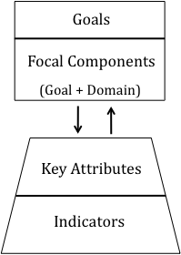
Figure 2. Proposed framework organization for assessing and reporting on ecosystem condition in Puget Sound.

The broadest category of division of our framework is Goals. Goals combine societal values and scientific understanding to define a desired ecosystem condition (Environmental Protection Agency 2002, Harwell et al. 1999). Explicit descriptions of the societal values related to the condition of Puget Sound are encompassed in the six statutory goals developed by the PSP (2009b), as shown in Section 3.1.3.

These goals reflect both societal and ecological interests in Puget Sound, and have been used as the fundamental organizing framework for assessing a ‘healthy’ Puget Sound ecosystem in the Partnership Action Agenda (Puget Sound Partnership 2009b). They are policy-relevant, which is foundational in the development of this framework. Note that for the purposes of indicator evaluation, we separated “Species” and “Food Webs.” This section focuses only on natural ecosystem components. Thus, human health and human well-being are addressed elsewhere in the PSSU.

Focal Components are the major ecological characteristics of an ecosystem that can be used to organize relevant information in a limited number of discrete, but not necessarily independent categories (Conservation Measures Partnership 2007). In the Open Standards for the Practice of Conservation they are referred to as, ‘focal conservation targets.’ The term ‘Focal Component’ has been used previously by the PSP (2009b) and has been adopted here to keep terminology consistent.

Focal Components were derived by dividing each of the Goals into distinct habitat domains that are characterized by unique qualities or traits. The domains we chose were marine, freshwater, terrestrial, and interface/ecotone. The interface/ecotone domain includes zones with a combination of traits from the other major groups such as the nearshore environment, wetlands, and estuaries.

This grouping (Table 2) provides a comprehensive view of the major ecological characteristics of Puget Sound based on area, and allows Focal Components to be assessed at an individual level (e.g., marine habitats), or aggregated into a single environment (e.g., assessing the integrity of the marine environment across all marine-related Focal Components).

Table 2. Summary of Focal Components based on goal and domain.

Goal	Domain	Focal Component
Species	Marine	Marine Species
	Freshwater	Freshwater Species
	Terrestrial	Terrestrial Species
	Interface/Ecotone	Interface Species
Food Webs	Marine	Marine Food Webs
	Freshwater	Freshwater Food Webs
	Terrestrial	Terrestrial Food Webs
	Interface/Ecotone	Interface Food Webs
Habitats	Marine	Marine Habitats
	Freshwater	Freshwater Habitats
	Terrestrial	Terrestrial Habitats
	Interface/Ecotone	Interface Habitats
Water Quality	Marine	Marine Water Quality
	Freshwater	Freshwater Quality
	Interface/Ecotone	Interface Water Quality
Water Quantity	Freshwater	Freshwater Quantity

Key Attributes are ecological characteristics that specifically describe the state of Focal Components. They are characteristic of the health and functioning of a focal component. They are explicitly defined based on each Focal Component and provide a clear and direct link between the Indicators and Focal Components. A similar tier has been identified by the PSP and others. A part of our framework development was an explicit comparison of the Key Attributes developed here with those suggested in the other reports. Although they differ in detail, the Key Attributes adopted here encompass all those identified by the Environmental Protection Agency (2002), Heinz Center (2008), and the PSP (2009b). Selected Key Attributes are shown in Table 3.

Table 3. Selected key attributes for each goal. Definitions (or measures) are meant to describe what is meant by each attribute. For example, population size is represented by the number of individuals in a population or the total biomass.

Goal	Key Attribute	Relevant Measures
Species	Population Size	Number of individuals or total biomass; Population dynamics
	Population Condition	Measures of population or organism condition including: Age structure; Population structure; Phenotypic diversity; Genetic diversity; Organism condition
Food Webs	Community Composition	Species diversity; Trophic diversity; Functional redundancy; Response diversity
	Energy and material flow	Primary production; Nutrient flow/cycling
Habitats	Habitat Area & Pattern/Structure	Area or extent; Measures of pattern/structure including: Number of habitat types; Number of patches of each habitat; Fractal dimension; Connectivity
	Habitat Condition	Abiotic & biotic properties of a habitat; Dynamic structural characteristics; Water & benthic condition
Water Quality	Hydrodynamics	Measures such as: Water movement; Vertical mixing; Stratification; Hydraulic residence time; Replacement time
	Physical/Chemical Parameters (Sediments & Water Column)	Measures such as: Nutrients; pH; Dissolved oxygen/redox potential; Salinity; Temperature
	Trace Inorganic & Organic Chemicals (Sediments & Water Column)	Measures such as: Toxic contaminants; Metals; Other trace elements & organic compounds
Water Quantity	Surface Water	Hydrologic Regime Measures such as: Flow magnitude & variability; Flood regime; Stormwater
	Groundwater Levels & Flow	Groundwater accretion to surface waters; Within groundwater flow rates & direction; Net recharge or withdrawals; Depth to groundwater
	Consumptive Water Use & Supply	Water storage

We reduced the list of potential attributes for each Goal and Focal Component to two or three Key Attributes for two reasons. First, this approach is driven by a need for simplicity, succinctness, and transparency in the development of an organizing framework. Second, the use of only 2-3 attributes for each Goal and Focal Component provides a means to address data gaps in the selection and evaluation of indicators. By defining the key attributes broadly, our framework allows for situations in which a single attribute (e.g., population condition for the Species Goal) can be informed by multiple types of indicators depending on information availability (e.g., population condition can be tracked using data on disease for some species, data on age structure for others, etc.).

A discussion of the Key Attributes for each goal follows.

A central goal identified by the PSP is to have ‘healthy and sustaining populations of native species in Puget Sound’ that provide ecosystem goods and services to humans, and support the structure and functioning of the ecosystem itself (Puget Sound Partnership 2008a). Many different attributes can describe whether a population is ‘healthy and sustaining’. For example, the U.S. Environmental Protection Agency (2002) identified eight different measures (i.e., attributes) of species condition including population size, genetic diversity, population structure, population dynamics, habitat suitability, physiological status, symptoms of disease or trauma, and signs of disease. Similar attributes identified by Fulton et al. (2005) included biomass, diversity, size structure, and spatial structure. Niemi and McDonald (2004) suggest attributes based on type, for example, structural attributes include genetic structure and population structure whereas functional attributes include life history, demographic processes, genetic processes, and behavior.

Historically the PSP has focused on population size as the species attribute, recognizing that species health or condition was encompassed by most other PSP goals (Puget Sound Action Team 2007a). More recently the PSP identified species key attributes by applying the Open Standards to the Action Agenda (Puget Sound Partnership 2009b). The species attributes they selected were forage fish, condition of key fish populations, population size and condition of key marine shellfish and invertebrates, population size and condition of key marine mammals, population size and condition of key marine birds, extent of all salmon species, condition of all listed salmon species, spatial structure of all listed salmon species, and population size and condition of key terrestrial bird species (Puget Sound Partnership 2009b).

Population size is defined as the number of individuals in a population or the total biomass of the population. Population dynamics that influence changes in abundance over time are also included. Population condition combines several measures: population structure, age structure, genetic diversity, phenotypic diversity, and organism condition.

Selection of Species Attributes in Puget Sound

Ecological attributes are intended to describe the state of an ecological system; in the case of species attributes, they are meant to describe the condition or viability of populations of species in an area. Measures of population condition or viability are important indicators, yet monitoring the status of all species is practically impossible. To address this, focus should be placed on identifying species indicators that characterize key interests in the region (i.e., focal species). For example, some species exert a disproportionately important influence on ecosystem condition, while others relate to biodiversity or are of direct interest to society. Examples of focal species include target, charismatic, vulnerable, and strongly interacting species. Target species are those fished or harvested for commercial gain or subsistence. Flagship species are those with widespread public appeal that are often used to communicate to the public about the condition of the ecosystem. Vulnerable species are those recognized with respect to their conservation status, for example, threatened, endangered, or of greatest conservation concern. Strongly interacting species (e.g., keystone species) are those whose presence, absence or rarity leads to significant changes in some feature of the ecosystem (adapted from Soulé et al. 2005 and Heiman 2005).

The following sections provide examples of the utility of population size and population condition in evaluating the status of focal species as well as ecosystem health.

Population size

Monitoring population size, in terms of total number of individuals or total biomass, is important for management and societal interests. For example, abundance estimates are used to track the status of threatened and endangered species and help determine whether a species is recovering or declining. Accurate estimates of population biomass of targeted fisheries species are used to assess stock viability and determine the number of fish that can be sustainably harvested from a region. While population size can be used to assess population viability, more accurate predictions of viability can be obtained by including the mechanisms responsible for the dynamics of the population. Population dynamics thus provide a predictive framework to evaluate the combined effect of multiple mechanisms of population regulation (e.g., birth and death rates, immigration and emigration) to evaluate changes in abundance through time.

Population condition

Whereas the preceding attribute is concerned with measures of population size, there are instances when the “health” of the population may be of interest. For example, monitoring changes in population condition may presage an effect on population size or provide insight into long-term population viability. The dynamics of many populations are better understood through knowledge of population condition such as organism condition, age structure, genetic diversity, phenotypic diversity, and population structure. Impaired condition of any or all of these subcategories indicates biological resources at risk. In addition, monitoring changes in organism condition can be used to infer changes in environmental conditions.

Organism condition

Organism condition represents both physiological and disease status. Monitoring organism condition may help predict changes in population size, and reveal environmental problems that warrant management action. Past efforts by the PSP have focused on organism condition (e.g., toxins in harbor seals) as an indicator of Water Quality. While this may be applicable for organisms at lower trophic levels (i.e., because they respond at shorter temporal scales), but time lags associated with the transfer of toxins through the food web means that higher trophic level organisms (e.g., killer whales, sixgill sharks) are unlikely to reveal Water Quality issues at time scales relevant to management. We suggest these measures (e.g., toxins in killer whales) are better served as an indicator of species population condition.

Physiological status is the key mechanism linking both organism and population to their environment (Wikelski and Cooke 2006). For example, individuals experiencing increased environmental stress may increase levels of stress hormones, eventually killing the individuals and leading to a decrease in population size. In the Galapagos, marine iguanas increased stress hormone levels due to fouling from an oil spill. The increase in stress hormone levels predicted a decrease in survival by approximately fifty percent, which was later confirmed by field studies (Wikelski et al. 2001). Disease status can affect population size and dynamics as well. In Prince William Sound, viral hemorrhagic septicemia virus (VHSV) was linked to a reduction in Pacific herring recruitment (Marty 2003). A recent paper by Landis and Bryant (2010) suggests that disease prevalence in Puget Sound was a contributing factor to the decline of Pacific herring (Cherry Point, Squaxin Pass, Discovery Bay, and Port Gamble stocks) in the 1970s and 1980s. Thus, monitoring organism condition may signal declines in population abundance before it occurs.

Monitoring organism condition is particularly important for long-lived organisms (e.g., marine mammals, rockfish) that live in contaminated habitats. Declines in population size of long-lived species may be slow to appear because of their long cohort turnover times. The temporal scale at which this occurs makes it difficult to recognize the population is in decline, and respond fast enough to prevent severe changes in population dynamics (Rowe 2008). Declining organism condition from contaminant exposure can also interact with diseases so that individuals in poor physiological condition are more susceptible to infections (Beldomenico and Begon 2010). In juvenile salmon, exposure to contaminants lead to increased disease susceptibility, significantly reducing population size (Arkoosh et al. 1998).

Finally, examining the physical condition of a population may reveal problems with current management strategies. For example, salmon injured by gillnets show reduced survival and fail to reproduce; this suggests estimates of spawning stocks, which count injured fish as part of the aggregate escapement of viable spawners, are inflated (Baker and Schindler 2009).

The remaining subcategories of population condition (i.e., age structure, population structure, genetic diversity, and phenotypic diversity) are primarily used for assessing focal species condition, and generally do not present information relating to environmental conditions. Due to this reason, these subcategories are discussed in terms of relevance to focal species.

Age structure

Population age structure is used to estimate population viability by modeling population trends through time, and can be especially useful for evaluating the long-term stability of a population. Monitoring age structure may also be useful in attributing declines in abundance to specific factors, which may otherwise be difficult to detect.

Robust age structure (i.e., multiple reproductive age classes) is critical for fish populations to withstand environmental variability and maintain resilience. Multiple reproductive age classes provide resilience for several reasons: (1) overall reproductive output increases, (2) age-related differences in spawning locations and timing allocate reproductive outputs across larger spatial and temporal areas, and (3) there is increased quantity and quality of eggs produced by older fish (Hsieh et al. 2010, Francis et al. 2007). Fisheries often target large and therefore old individuals, effectively truncating the age structure of the population. This is likely to reduce population resilience.

In order to attribute declines in stellar sea lion (SSL) populations to specific factors, age-structure information is required to separate out vital rate changes from population abundance estimates (Holmes et al. 2007). For example, a risk factor (e.g., contaminants) may affect an age-specific vital rate but show no corresponding change in population abundance. Examining age-structure trends may provide insight into population declines of various species in Puget Sound (e.g., Southern Resident Killer Whales, Pacific herring, rockfish) or elucidate factors that affect age-specific organism condition.

Genetic diversity

Genetic diversity measures may be important in assessing long-term population viability, as well as the ability for a population to adapt to changing environmental conditions. Monitoring genetic loci or gene expression may also help detect the onset of selection events such as emerging diseases, climate change or land use change, or pollution (Schwartz et al. 2007).

Although not always the case (Levin and Schiewe 2001), loss of genetic variation can reduce individual fitness (e.g., through loss of heterozygosity), as well as the ability of populations to evolve in the future (e.g., through loss of allelic diversity) (Allendorf, F.W., et al. 2008. Genetic effects of harvest on wild animal populations. Trends in Ecology & Evolution 23(6):327-337.). For example, in Greater Prairie Chickens loss of genetic variation was linked with lower hatching success of eggs following population declines (Westemeier et al. 1998). Genetic changes (e.g., declines in fecundity, egg volume, larval size, etc.) caused by overharvesting fish populations can increase extinction risks and reduce the capacity for population recovery (Walsh et al. 2006).

Phenotypic diversity

Individual organisms adapt to changing environmental conditions by sensing the changes and responding appropriately, for instance, by switching their behavior or physiology. However this means that every individual must reserve a portion of their energy to actively sensing and adapting to environmental changes. An alternative strategy is to diversify a population: each subset of the total population is adapted to a slightly different environmental condition (i.e., phenotypic diversity). Sockeye salmon, for example, show a suite of adaptations to the diversity of spawning habitats. This phenotypic diversity has proven to be critical under changing environmental conditions in Bristol Bay, Alaska. As conditions changed, populations demonstrated differential responses so that at different times, different populations became more productive (Hilborn et al. 2003a). In California, the development of the Sacramento-San Joaquin watershed has truncated the life history diversity of Chinook salmon, resulting in the collapse of these populations (Lindley et al. 2009). Recognizing and understanding phenotypic diversity may prevent the loss of population subsets that currently appear unproductive, but may prove vital for long-term population sustainability.

Population structure

Population structure refers to spatial dynamics, or how different populations interact in space. In many instances local populations are linked, thereby creating a metapopulation. When environmental conditions change, some populations decline while others persist, but the overall density of the metapopulation may remain relatively steady. Metapopulations persist through a suite of adaptations at the individual (e.g., physiological and behavioral adaptations) and population level (e.g., each subpopulation lives in a separate location and contains distinct demographic parameters). Understanding the spatial variation of populations, how they interact, and how demographic parameters differ among these populations are essential to sound management of focal species.

For example, sedentary stocks such as benthic invertebrates are typically structured as metapopulations; the subpopulations stay connected through larval or juvenile dispersal. The strong spatial effects not only make it difficult for a population to persist on its own, but adding in pressure from fishing has the chance to lead to stock depletion (Hilborn et al. 2003b). In Bristol Bay, sockeye salmon populations exist as mixed stocks (i.e., a metapopulation stock complex) during their adult phase. Management of salmon has historically focused on the metapopulation stock complex, rather than concentrating on the most productive populations. As a result, sockeye salmon harvest has remained relatively stable over decades. In the conservation of threatened species it is important to recognize that single populations have a high risk of extinction, and effectively managing for species persistence requires a metapopulation-level approach. For example, recovery strategies for Puget Sound Chinook salmon recommend two to four viable subpopulations within each geographic region to reduce the risk of extinction for the metapopulation (Puget Sound Technical Recovery Team 2002).

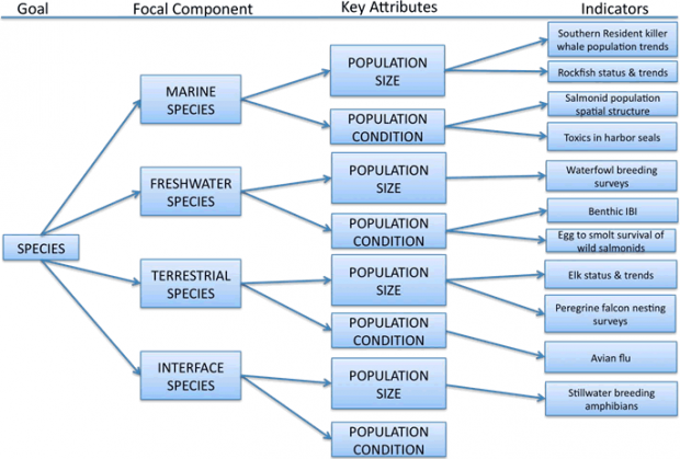
Figure 3. Summary of framework organization for Species goal. The list of indicators is illustrative only, and not complete.

The food web indicator evaluations focused on two key attributes: (1) community composition, and (2) energetics and material flows. These two attributes reflect the structure and function of a food web and were drawn from a large literature on the subject (Environmental Protection Agency 2002, Pimm 1984, Odum 1969, Odum 1985, Pacala and Kinzig 2002, Srivastava and Vellend 2005, Williams and Martinez 2000). Food web attributes provide a measure of the extent to which different components of the ecosystem interact (e.g., habitats and species) along with important contextual information for understanding the status of the individual components themselves.

We have adopted a broad definition of community composition that includes species diversity, trophic diversity, functional redundancy, and response diversity. This definition is consistent with “community attributes,” a key attribute for food webs recently designated by the PSP (2009b). Species diversity encompasses species richness, or the number of species, in the food web, and species evenness, or how individuals or biomass are distributed among species within the food web (Pimm 1984). Trophic diversity refers to the relative abundance or biomass of different primary producers and consumers within a food web (Environmental Protection Agency 2002). Consumers include herbivores, carnivores or predators, omnivores, and scavengers. Functional redundancy refers to the number of species characterized by traits that contribute to a specific ecosystem function, whereas response diversity describes how functionally similar species respond differently to disturbance (Laliberte and Legendre 2010). For example, a food web containing several species of herbivores would be considered to have high functional redundancy with respect to the ecosystem function of grazing, but only if those herbivorous species responded differently to the same perturbation (e.g., trawling) would the food web be considered to have high response diversity.

Like community composition, the second key attribute of food webs, energy and material flows, was previously highlighted by the PSP (2009b). This attribute includes ecological processes such as primary production and nutrient cycling, in addition to flows of organic and inorganic matter throughout a food web. Primary productivity is the capture and conversion of energy from sunlight into organic matter by autotrophs, and provides the fuel fundamental to all other trophic transfer in a food web. Material flows, or the cycling of organic matter and inorganic nutrients (e.g., nitrogen, phosphorus), describe the efficiency with which a food web maintains its structure and function.

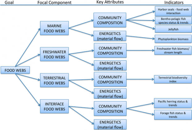
Figure 4. Summary of framework organization for Food Webs goal. The list of indicators is illustrative only, and not complete.

The Puget Sound basin encompasses diverse marine, nearshore, freshwater, and terrestrial habitats. As such, a key goal of the PSP is to have ‘a healthy Puget Sound where freshwater, estuary, nearshore, marine, and upland habitats are protected, restored, and sustained’ (from RCW 90.71.300). Many different ecological attributes may be used to describe habitat status and determine whether or not it is ‘healthy’. The U.S. EPA (2002) identified various attributes of habitats (referred to as ‘landscapes’) including extent, composition, and pattern/structure; other attributes of habitats included dynamic structural characteristics and physical structure. The U.S. EPA (2002) also acknowledged habitat condition, but recommended its use as a species attribute (i.e., habitat suitability) because they defined condition in terms of the organisms of interest. Similar landscape attributes identified by the Heinz Center (2008) included extent and pattern.

In 2009, the PSP structured their reporting on ecosystem status around two broad indicator categories for the habitat goal: extent and condition of ecological systems. These broad categories were selected to represent key attributes associated with the habitat goal (Puget Sound Partnership 2009b), and were used to report on extent and condition of focal habitats in Puget Sound (Puget Sound Partnership 2009c). Simultaneously, a PSP working group identified several key habitat attributes including: estuarine wetlands, delta or river mouth condition, coastal embayments and lagoons, forage fish spawning habitat/substrate, condition of shorelines and condition of beaches, benthic condition, marine water condition, freshwater condition, spatial extent of ecological systems (terrestrial), condition of ecological systems or plant associations (terrestrial), and functional condition for key terrestrial species (Puget Sound Partnership 2009b).

 

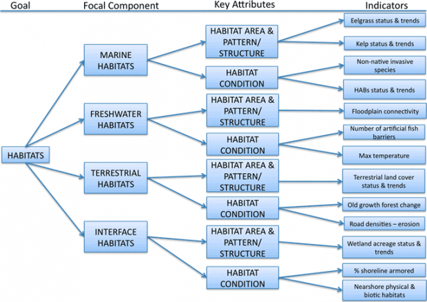
Figure 5. Summary of framework organization for Habitats goal. The list of indicators is illustrative only, and not complete.

Habitat area and pattern/structure combines several measures. Habitat area is defined as the areal extent and shape of each habitat type. Pattern/structure refers to the number of habitat types, the number of patches of each habitat, fractal dimension (i.e., habitat complexity), and connectivity. Habitat condition refers to abiotic properties (i.e., physical and chemical properties) and biotic properties (e.g., invasive or nuisance species, dominant species). Dynamic structural characteristics (i.e., changes in physical habitat complexity and morphology) are also included in habitat condition because they maintain the diversity of natural habitats. Water quality and benthic condition also contribute to habitat condition; however, according to the PSSU framework, they fall under the Water Quality goal and will therefore be discussed in that section.

The purpose of the framework development with regard to indicator selection, was to ensure that there was complete coverage of the goals by the indicators. The first division of goals was into ecologically unique domains (e.g., marine water, freshwater, and ecotones), which defined the Key Attributes. The properties of the Key Attributes must be known in order to define the state of that aspect of the ecosystem. Key attributes must be managed in order to sustain each conservation target (i.e. focal components) (Parrish et al. 2003, The Nature Conservancy 2007). This approach is similar to that previously utilized by the PSP (2009b).

There are three key attributes, which articulate Water Quality: hydrodynamics, the physical and chemical parameters, and trace inorganic and organic contaminants. These key attributes for water quality have also been utilized elsewhere (Environmental Protection Agency 2002, Harwell et al. 1999, Fancy et al. 2009).

Hydrodynamics are important characteristics of water quality in marine, freshwater, and transitional (e.g., wetlands, estuaries, etc.) systems. River and stream hydrodynamics are defined by various aspects of the flow regime including magnitude, frequency, duration, timing, and rate of change. Each of these has important impacts on ecology and human health and well-being (Poff et al. 1997, Poff  and Zimmerman 2010, Fu et al. 2010, Barnett et al. 2008). The hydrodynamics of river and stream is discussed in the Water Quantity section of this Puget Sound Science Update. Lake hydrodynamics are generally defined by mixing, stratification (i.e. the lack of mixing), and residence times. All of these are key aspects of nutrient cycling and can be deterministic in lake water quality (Arhonditsis, G.B. and M.T. Brett. 2005. Eutrophication model for Lake Washington (USA) Part I. Model description and sensitivity analysis. Ecological Modelling 187(2-3):140-178., Hamilton and Schladow 1997). Hydrodynamics are also important in marine environments. Offshore circulation patterns and seawater intrusions into Puget Sound bring in nutrient rich waters, which can impact eutrophication and dissolved oxygen (see Chapter 6 of the Puget Sound Science Review; (Mackas and Harrison 1997, Connolly et al. 2010, Leonov and Kawase 2009, Moore et al. 2008a, Moore et al. 2008b)). Rivers and streams entering Puget Sound create areas of density stratification, which can also affect eutrophication (Moore et al. 2008b, Paulson et al. 1993). Hydrodynamics are critical in understanding water quality and have been incorporated as a Key Attribute.

Physical and chemical parameters are also crucial in determining water quality. The suitability of freshwater and marine water systems to support biota is strongly dependent on temperature and dissolved oxygen (DO; see Washington State Department of Ecology 2002a, Washington State Department of Ecology 2002b and references therein). Low DO is an issue of management importance in the Hood Canal and the south Puget Sound (Puget Sound Partnership 2009d). The level of nutrients such as nitrogen and phosphorus in lakes and estuaries can affect primary productivity and habitat quality (Mackas and Harrison 1997, Bernhard and Peele 1997, Carlson 1977, Edmondson 1970, Edmonson 1994, Edmondson and Lehman 1981, Howarth and Marino 2006, Smith 2003). Anthropogenic nutrient inputs have been associated with harmful algal blooms (see Chapter 5 of the Puget Sound Science Review; Anderson, D.M., et al. 2008. Harmful algal blooms and eutrophication: Examining linkages from selected coastal regions of the United States. Harmful Algae 8(1):39-53). Increasing levels of atmospheric carbon dioxide in the may lead to decreased pH with ocean acidification, potentially resulting in severe impacts on key marine organisms with calcium carbonate exoskeletons (Orr et al. 2005). General physical and chemical parameters are of import in defining water quality and are, thus, utilized as Key Attributes.

The presence and concentrations of trace organic and inorganic chemicals, also known as toxics, contaminants, pollutants, etc., may have impacts of the human health and the environment. Much of the implementation of the Clean Water Act has focused on the reduction of chemicals into surface waters for "the protection and propagation of fish, shellfish, and wildlife and recreation in and on the water" (Federal Water Pollution Control Act 2002). A discussion of the toxic contaminants in Puget Sound is included in Chapter 5 of this Puget Sound Science Review. Due to their potential importance both ecologically and to human-well being, trace organic and inorganic chemicals is a Key Attribute of water quality.

Figure 6. Summary of framework organization for Water Quality goal. The list of indicators is illustrative only, and not complete.

In order to evaluate indicators of water quantity, we used three distinct Key Attributes: the surface water hydrologic regime, groundwater levels and flows, and consumptive water use and supply. The PSP has utilized other organizational frameworks though they selected similar attributes. In the 2009 document, “Identification of Ecosystem Components and Their Indicators and Targets,” water quantity was not dealt with as an explicit goal but rather as supportive of habitats and human uses (Puget Sound Partnership 2009b). This resulted in the selection of freshwater extent, freshwater condition, and water supply for end users as attributes – all similar to the Key Attributes used herein. The EPA defined surface and groundwater flows as an essential ecosystem attribute category with subcategories including pattern of surface flows, hydrodynamics, and pattern of groundwater flows (Environmental Protection Agency 2002). Their framework focused on ecological condition and did not explicitly include human dimensions. The Heinz Center (2008) reports on the extent of freshwater ecosystems, changing stream flows, water withdrawals, and groundwater levels. Other studies have reported the use of similar attributes to define the state of water quantity (Walmsley 2002).

The surface water hydrologic regime has important impacts on the regional ecosystems (see Poff et al. 1997 and references, therein). The groundwater is an important source both for consumptive use and river and stream base-flows. Consumptive water use and supply are important measures of resource conservation and supply and relate strongly to the human health and well-being of the region.

Figure 7. Summary of framework organization for Water Quantity goal. The list of indicators is illustrative only, and not complete.

Indicators are metrics that reflect the structure, composition, or functioning of an ecological system (Environmental Protection Agency 2002, Heinz Center 2008). Indicators are measurable characteristics that can assess changes in ecosystem attributes. A list of candidate indicators was selected from several sources (see Section 4.1) and each indicator was assigned to a specific Key Attribute based on expert opinion. Indicator identification and evaluation is discussed in Section 4.

A conceptual framework for selecting indicators of ecosystem condition is valuable for several reasons. First, indicators are often selected based on the degree to which they meet a number of criteria individually, rather than on the basis of how they collectively assess ecosystem condition (Niemeijer and de Groot 2008). A conceptual framework explicitly includes the inter-relation of indicators as part of the indicator selection process, and helps to develop consistent indicator sets (Niemeijer and de Groot 2008). Second, a conceptual framework provides flexibility. For example, if the goal is to assess marine ecosystem health using only ten indicators, a hierarchical framework provides a way to select indicators so that all the relevant ecosystem components are included. In this case, one to three indicators would be selected from Marine Species, Marine Food Webs, Marine Habitats, and Marine Water Quality in order to ensure adequate representation of all the important features. Third, a framework highlights indicators that may be relevant to multiple goals, focal components, or attributes. For example, the population abundance of Western sandpipers is related to the Species goal, but may also be relevant to the Habitats goal if their abundance reflects changes in habitat condition. Finally, a framework explicitly links indicators→attributes→ focal components→goals, which ensures sufficient coverage of the Key Attributes essential to each goal. A conceptual framework provides a structured yet flexible way to select indicators that best represent the environmental issue at hand.

Key point: A carefully crafted framework provides a robust means for assuring that ecosystem indicators are explicitly linked to societal goals. The approach we present melds a number of separate PSP activities into a single, transparent framework and provides a structured yet flexible means to select ecologically and socially meaningful indicators.

Allendorf, F.W., et al. 2008. Genetic effects of harvest on wild animal populations. Trends in Ecology & Evolution 23(6):327-337.

Anderson, D.M., et al. 2008. Harmful algal blooms and eutrophication: Examining linkages from selected coastal regions of the United States. Harmful Algae 8(1):39-53.

Arhonditsis, G.B. and M.T. Brett. 2005. Eutrophication model for Lake Washington (USA) Part I. Model description and sensitivity analysis. Ecological Modelling 187(2-3):140-178.

Arkoosh, M.R., et al. 1998. Effect of pollution on fish diseases: Potential impacts on salmonid populations. Journal of Aquatic Animal Health 10(2):182-190.

Baker, M.R. and D.E. Schindler. 2009. Unaccounted mortality in salmon fisheries: non-retention in gillnets and effects on estimates of spawners. Journal of Applied Ecology 46(4):752-761.

Barnett, T.P., et al. 2008. Human-induced changes in the hydrology of the western United States. Science 319(5866):1080-1083.

Beldomenico, P.M. and M. Begon. 2010. Disease spread, susceptibility and infection intensity: vicious circles? Trends in Ecology & Evolution 25(1):21-27.

Bernhard, A.E. and E.R. Peele. 1997. Nitrogen limitation of phytoplankton in a shallow embayment in northern Puget Sound. Estuaries 20(4):759-769.

Carlson, R.E. 1977. TROPHIC STATE INDEX FOR LAKES. Limnology and Oceanography 22(2):361-369.

Connolly, T.P., et al. 2010. Processes influencing seasonal hypoxia in the northern California Current System. Journal of Geophysical Research-Oceans 115.

Conservation Measures Partnership. 2007. Open Standards for the Practice of Conservation, Version 2.0.

Edmondson, W.T. 1970. PHOSPHORUS, NITROGEN, AND ALGAE IN LAKE WASHINGTON AFTER DIVERSION OF SEWAGE. Science 169(3946):690-691.

Edmondson, W.T. 1994. Sixty Years of Lake Washington: a Curriculum Vitae. Lake and Reservoir Management 10(2):75 - 84.

Edmondson, W.T. and J.T. Lehman. 1981. THE EFFECT OF CHANGES IN THE NUTRIENT INCOME ON THE CONDITION OF LAKE WASHINGTON. Limnology and Oceanography 26(1):1-29.

Environmental Protection Agency. 2002. A Framework for Assessing and Reporting on Ecological Condition: A Science Advisory Board Report, T.F. Young and S. Sanzone, Editors. Washington, D.C.

Environmental Protection Agency. 2008. EPA’s 2008 Report on the Environment. National Center for Environmental Assessment, Washington, DC. EPA/600/R-07/045F.

Environmental Protection Agency. 2010. Puget Sound Georgia Basin Ecosystem Indicators. Available from: http://www.epa.gov/pugetsound/indicators/index.html.     

Fancy, S.G., J.E. Gross, and S.L. Carter. 2009. Monitoring the condition of natural resources in US national parks. Environmental Monitoring and Assessment 151(1-4):161-174.

Federal Water Pollution Control Act. 2002. Title 33, Chapter 26, Subchapter 1251. As Amended 2002: United States.

Fleishman, E. and D.D. Murphy. 2009. A realistic assessment of the indicator potential of butterflies and other charismatic taxonomic groups. Conservation Biology 23(5):1109-1116.

Francis, R.C., et al. 2007. Fisheries management - Ten commandments for ecosystem-based fisheries scientists. Fisheries 32(5):217-233.

Fu, G.B., M.E. Barber, and S.L. Chen. 2010. Hydro-climatic variability and trends in Washington State for the last 50 years. Hydrological Processes 24(7):866-878.

Fulton, E.A., A.D.M. Smith, and A.E. Punt. 2005. Which ecological indicators can robustly detect effects of fishing? ICES Journal of Marine Science 62(3):540-551

Hamilton, D.P. and S.G. Schladow. 1997. Prediction of water quality in lakes and reservoirs. Model description. Ecological Modelling 96(1-3):91-110.

Harwell, M.A., et al. 1999. A framework for an ecosystem integrity report card. Bioscience 49(7):543-556.

Heiman, K. 2005. Strongly interacting nonindigenous species. Bioscience 55(7):548-548.

Heinz Center. 2008. The State of the Nation's Ecosystems 2008: Measuring the Lands, Waters, and Living Resources of the United States. Washington, DC: Island Press.

Hilborn, R., et al. 2003a. Biocomplexity and fisheries sustainability. Proceedings of the National Academy of Sciences of the United States of America 100(11):6564-6568.

Hilborn, R., et al. 2003b. State of the world's fisheries. Annual Review of Environment and Resources 28:359-399.

Holmes, E.E., et al. 2007. Age-structured modeling reveals long-term declines in the natality of western Steller sea lions. Ecological Applications 17(8):2214-2232.

Howarth, R.W. and R. Marino. 2006. Nitrogen as the limiting nutrient for eutrophication in coastal marine ecosystems: Evolving views over three decades. Limnology and Oceanography 51(1):364-376.

Hsieh, C.H., et al. 2010. Fishing effects on age and spatial structures undermine population stability of fishes. Aquatic Sciences 72(2):165-178.

Kurtz, J.C., L.E. Jackson, and W.S. Fisher. 2001. Strategies for evaluating indicators based on guidelines from the Environmental Protection Agency’s Office of Research and Development. Ecological Indicators 1(1): 49-60.

Laliberte, E. and P. Legendre. 2010. A distance-based framework for measuring functional diversity from multiple traits. Ecology 91(1):299-305.

Landis, W.G. and P.T. Bryant. 2010. Using weight of evidence characterization and modeling to investigate the cause of the changes in Pacific herring (Clupea pallasi) population dynamics in Puget Sound and at Cherry Point, WA. Risk Analysis 30(2):183-202.

Landres, P.B., J. Verner, and J.W. Thomas. 1988. ECOLOGICAL USES OF VERTEBRATE INDICATOR SPECIES - A CRITIQUE. Conservation Biology 2(4):316-328.

Leonov, D. and M. Kawase. 2009. Sill dynamics and fjord deep water renewal: Idealized modeling study. Continental Shelf Research 29(1):221-233.

Levin, P., et al. 2008. Integrated ecosystem assessments. National Oceanic and Atmospheric Administration. Seattle (WA).

Levin, P.S. and M.S. Schiewe. 2001. Preserving salmon biodiversity. American Scientist 89:220-228.

Lindley, S.T., et al. 2009. What caused the Sacramento River fall Chinook stock collapse? Pacific Fishery Management Council.

Mackas, D.L. and P.J. Harrison. 1997. Nitrogenous nutrient sources and sinks in the Juan de Fuca Strait of Georgia Puget Sound estuarine system: Assessing the potential for eutrophication. Estuarine Coastal and Shelf Science 44(1):1-21.

Marty, G.D., et al. 2003. Role of disease in abundance of a Pacific herring (Clupea pallasi) population. Canadian Journal of Fisheries and Aquatic Sciences 60(10):1258-1265.

Moore, S.K., et al. 2008a. Local and large-scale climate forcing of Puget Sound oceanographic properties on seasonal to interdecadal timescales. Limnology and Oceanography 53(5):1746-1758.

Moore, S.K., et al. 2008b. A descriptive analysis of temporal and spatial patterns of variability in Puget Sound oceanographic properties. Estuarine Coastal and Shelf Science 80(4):545-554.

Niemeijer, D. and R.S. de Groot. 2008. A conceptual framework for selecting environmental indicator sets. Ecological Indicators 8(1):14-25.

Niemi, G.J. and M.E. McDonald. 2004. Application of ecological indicators. Annual Review of Ecology Evolution and Systematics 35:89-111.

Odum, E.P. 1969. Strategy of ecosystem development. Science 164(3877):262-270.

Odum, E.P. 1985. Trends expected in stressed ecosystems. BioScience 35(7):419-422.

O'Neill, S.M., C.F. Bravo, and T.K. Collier. 2008. Environmental Indicators for the Puget Sound Partnership: A Regional Effort to Select Provisional Indicators (Phase 1). Summary Report. National Oceanic and Atmospheric Administration. Seattle (WA).

Orr, J.C., et al. 2005. Anthropogenic ocean acidification over the twenty-first century and its impact on calcifying organisms. Nature 437(7059):681-686.

Pacala, S. and A. Kinzig. 2002. Introduction to theory and the common ecosystem model. In: A. Kinzig, S. Pacala, and D. Tilman, Editors. Functional consequences of biodiversity: empirical progress and theoretical extensions. Princeton (NJ): Princeton University Press. p. 169-174.    

Parrish, J.D., D.P. Braun, and R.S. Unnasch. 2003. Are we conserving what we say we are? Measuring ecological integrity within protected areas. Bioscience 53(9):851-860.

Paulson, A.J., H.C. Curl, and R.A. Feely. 1993. The Biogeochemistry of Nutrients and Trace-Metals In Hood Canal, A Puget-Sound Fjord. Marine Chemistry 43(1-4):157-173.

Pimm, S.L. 1984. The complexity and stability of ecosystems. Nature 307(5949):321-326.

Poff, N.L., et al. 1997. The natural flow regime. Bioscience 47(11):769-784.

Poff, N.L. and J.K.H. Zimmerman. 2010. Ecological responses to altered flow regimes: a literature review to inform the science and management of environmental flows. Freshwater Biology 55(1):194-205.

Puget Sound Action Team. 2007a. 2007 Puget Sound Update: Ninth Report of the Puget Sound Assessment and Monitoring Program. Olympia (WA). p. 260.

Puget Sound Ambient Monitoring Program. 2000. A conceptual model for environmental monitoring of a marine system. Washington Department of Fish and Wildlife.

Puget Sound Ambient Monitoring Program. 2010. Washington Department of Fish and Wildlife. Available from: http://wdfw.wa.gov/conservation/research/projects/marine_toxics/.

Puget Sound Nearshore Ecosystem Restoration Project. 2006. Conceptual model for assessing restoration of Puget Sound nearshore ecosystem. University of Washington. Seattle (WA).

Puget Sound Partnership. 2008a. Puget Sound Action Agenda, Protecting and Restoring the Puget Sound Ecosystem by 2020. Olympia (WA).

Puget Sound Partnership. 2009b. Identification of Ecosystem Components and Their Indicators and Targets. Puget Sound Partnership.

Puget Sound Partnership. 2009c. Ecosystem Status and Trends. Puget Sound Partnership.

Puget Sound Technical Recovery Team. 2002. Planning ranges and preliminary guidelines for the delisting and recovery of the Puget Sound Chinook salmon evolutionarily significant unit.

Rice, J.C. and M.-J. Rochet. 2005. A framework for selecting a suite of indicators for fisheries management. ICES J. Mar. Sci. 62(3):516-527.

Rowe, C.L. 2008. "The Calamity of So Long Life": Life histories, contaminants, and potential emerging threats to long-lived vertebrates. Bioscience 58(7):623-631.

Schwartz, M.K., G. Luikart, and R.S. Waples. 2007. Genetic monitoring as a promising tool for conservation and management. Trends in Ecology & Evolution 22(1):25-33.

Smith, V.H. 2003. Eutrophication of freshwater and coastal marine ecosystems - A global problem. Environmental Science and Pollution Research 10(2):126-139.

Soulé, M.E., et al. 2005. Strongly interacting species: conservation policy, management, and ethics. Bioscience 55(2):168-176.  

Srivastava, D.S. and M. Vellend. 2005. Biodiversity-ecosystem function research: is it relevant to conservation? Annual Review of Ecology, Evolution, and Systematics 36:267-294.

The Nature Conservancy. 2007. Advanced Guidance for Step 3: Assessing the Viability of the Focal Conservation Targets. The Nature Conservancy.

Walmsley, J.J. 2002. Framework for measuring sustainable development in catchment systems. Environmental Management 29(2):195-206.

Walsh, M.R., et al. 2006. Maladaptive changes in multiple traits caused by fishing: impediments to population recovery. Ecology Letters 9(2):142-148.

Washington State Department of Ecology. 2002a. Evaluating Criteria for the Protection of Freshwater Aquatic Life in Washington’s Surface Water Quality Standards: Dissolved Oxygen. Draft Discussion Paper and Literature Summary. Washington State Department of Ecology. Olympia (WA). p. 90.

Washington State Department of Ecology. 2002b. Evaluating Standards for Protecting Aquatic Life in Washington's Surface Water Quality Standards: Temperature Criteria. Draft Discussion Paper and Literature Summary. Washington State Department of Ecology. Olympia (WA).

Westemeier, R.L., et al. 1998. Tracking the long-term decline and recovery of an isolated population. Science 282(5394):1695-1698.

Wikelski, M., L.M. Romero, and H.L. Snell. 2001. Marine Iguanas Oiled in the Galapagos. Science 292(5516):437-438.

Wikelski, M. and S.J. Cooke. 2006. Conservation physiology. Trends in Ecology & Evolution 21(1):38-46.

Williams, R.J. and N.D. Martinez. 2000. Simple rules yield complex food webs. Nature 404(6774):180-183.